Time Series Analysis Walmart Sales Forecasting

Overview

This project focuses on forecasting retail sales using time series models. We analyze Walmart’s hierarchical sales data to predict future weekly sales trend, by implementing ARIMA/SARMIMA and Gaussian Processes (GP). We also aim to evaluate the models based on their accuracy, robustness, and computational efficiency.

Dataset

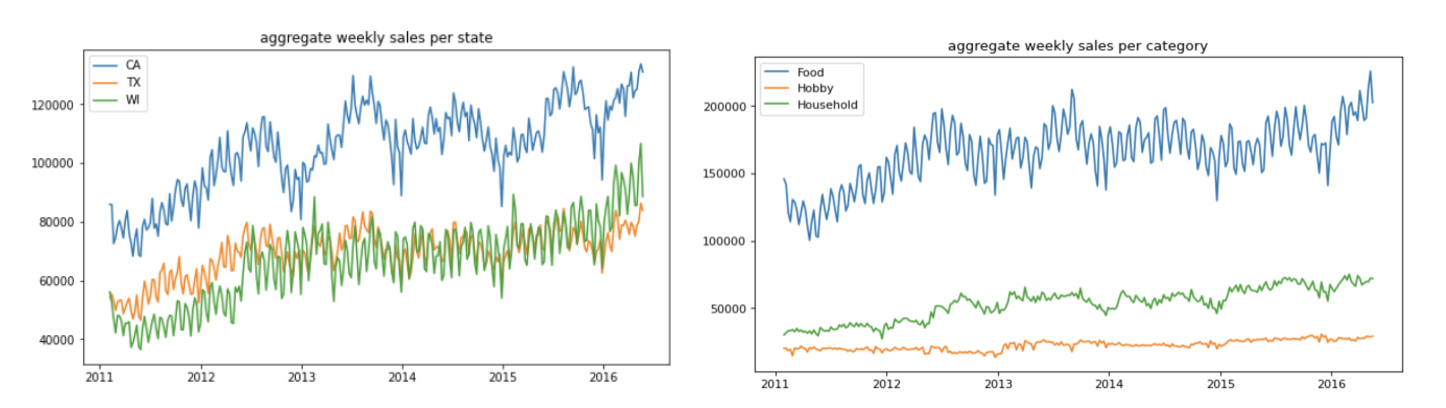
The dataset we use is hierarchical sales data from Walmart Daily Sales ranging from Jan 28th 2011 to Jun 18th 2016, containing sales information of products in three categories (Food, Hobby, Household) sold in three states (California, Texas, Wisconsin). For prediction, we aggregate the daily sales into weekly sales data in three categories sold in three states.

Methodology

We use drill-down analysis to dissect the data at a more granular level: for each category and each state, we compare ARIMA/SARMIA and GP model’s performance on our test data using RMSE metric for best model selection.

Data Preprocessing

• Aggregate daily sales to weekly for forecasting with pandas groupby, reduing noise and making patterns more discernable
• Remove the first week of sales data as it did not represent a full week to avoid skewing the model
• Divide the dataset into training (first 267 weeks) and test (last 10 weeks) sets to evaluate the performance of our time series models

Model Selection

Why ARIMA/SARIMA?

• Rationale: ARIMA(AutoRegressive Integrated Moving Average) and SARIMA (Seasonal ARIMA) are powerful and widely used statistical models for time series forecasting that can capture both trend and seasonality in the dataset.
• Model Explained:
  • ARIMA models are characterized by three main hyperparameters: (p, d, q):
    • p is the order of the AutoRegressive (AR) part, the number of lagged observations
    • d is the degree of differencing required to make the time series stationary
    • q is the order of the Moving Average (MA) part, the size of the moving average window
  • SARIMA extends ARIMA by adding additional seasonal terms: (P, D, Q)m:
    • P, D, and Q represent the seasonal components of the AR, differencing, and MA parts, respectively
    • m refers to the number of periods in each season
• Implementation Steps:
  • Stationary Check: We conduct the Augmented Dickey-Fuller (ADF) test to ensure that the time series is stationary (if p-value is less than significant level, we can reject the null hypothesis and take that the series is stationary).
  • ACF/PACF Plots: We use these plots to select ARIMA/SARIMA model hyperparameters.
  • Parameter Optimization: We use grid search to identify the best of hyperparameters that minimize information crtieria such as AIC.

Why Gaussian Processes (GP)?

• Rationale: GPs use Bayesian inference to make forecasts, which are suitable for datasets with complex dependencies and latent dynamics
• Implementation Steps:
  • Kernel Selection: To determine the appropriate kernel functions, we observe that our data has 1) an increasing trend 2) some form of periodicity. Thus, two main kernels we use are exponential squared (RBF) kernel and periodic kernel.
  • Hyperparameter Tuning: We optimize kernel hyperparameters to maximize the log-marginal likelihood, ensuring the model fits the data effectively.

Results

We use RMSE (normalized) to evaluate the model performance as the following:

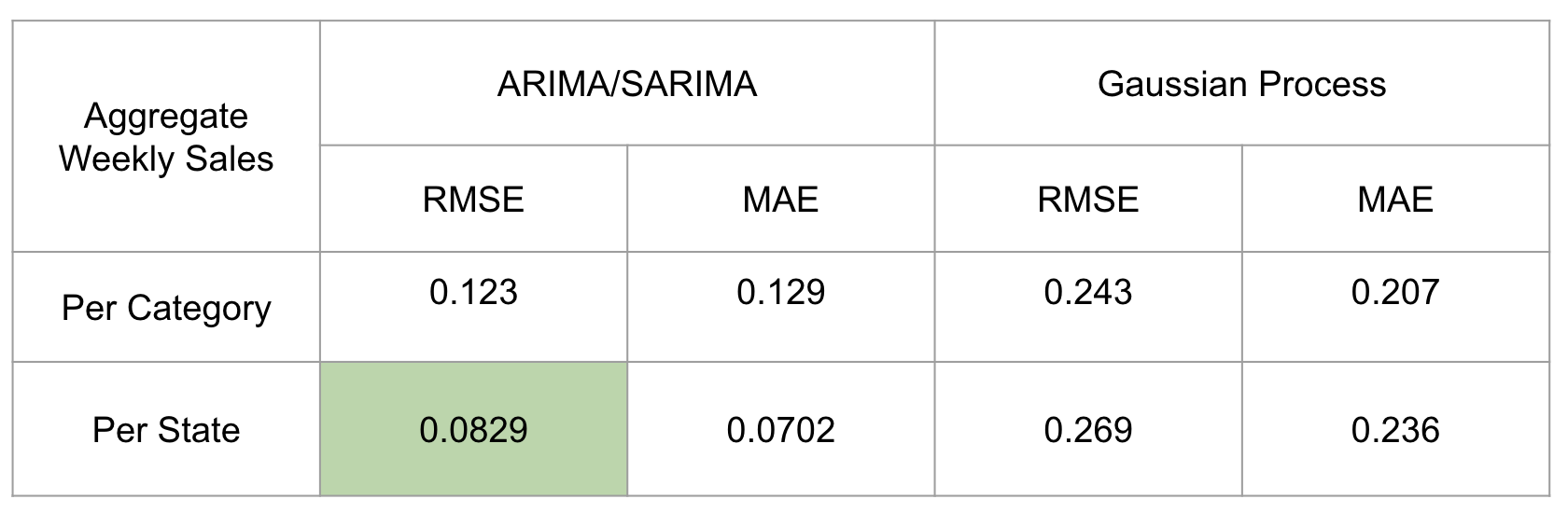
The MAPE (mean absolute percentage error) is 2.31% for ARIMA/SARIMA and 5.08% for GPs.

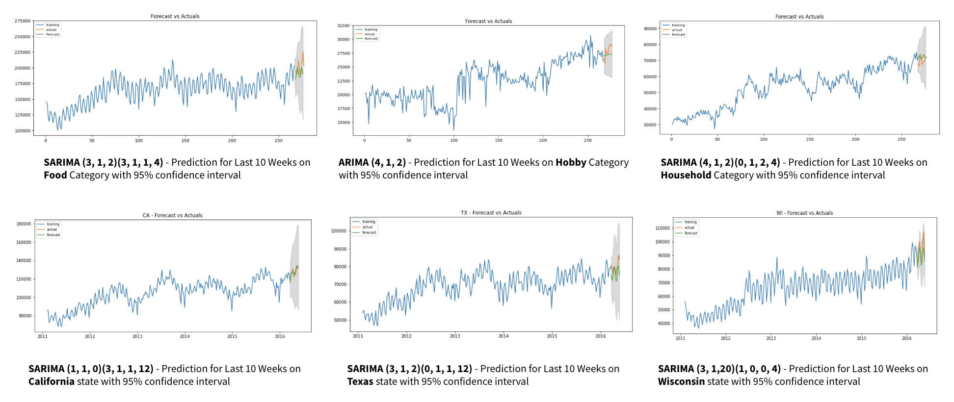
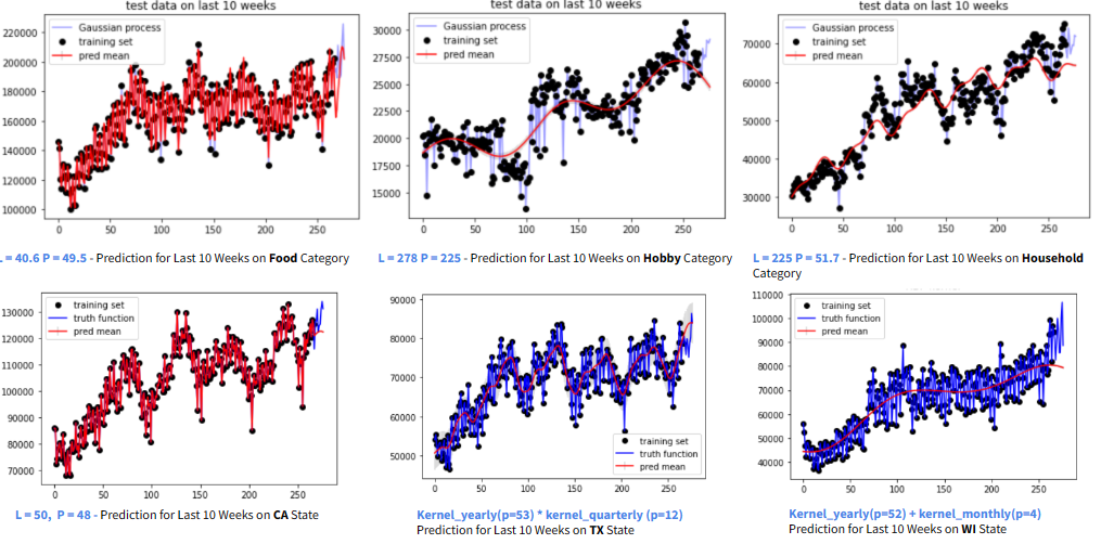
Here is the prediction plot by using ARIMA/SARIMA and GP:

Conclusion

The project confirms the efficiency of ARIMA/SARIMA models for time series forecasting in retail sales. While GPs provide flexibility, their higher computational cost and complexity in hyperparameter tuning make ARIMA/SARIMA a more practical choice for this application. Future work will include integrating external datasets like holidays to account for sales variability during special days and exploring other robust forecasting models, such as LSTM.